Module 1: The Basics

Before we can really talk about building and assessing statistical models with data, you will need to be familiar with some basics of probability theory, coding, and simulation. This module will provide these basics as well as motivate why our framework for confronting data from a statistical viewpoint is justified. You will quickly see that while some of these basics resemble what you might learn in an introductory statistics textbook, our emphasis will reside much more on the practical and intuitive aspects of probability rather than on developing a series of rules and tests. In particular, we believe that a modern quantitative thinker knows not just the theory of what a probability density function is (for example), but also how to generate one from data or simulations, how to visualize one, and how to manipulate one to make different calculations.

These notes have three sections: the first section will simply link to the Python tutorial that should be completed before/during the reading of this text. The next two sections will then introduce basic probability concepts, such as probability and frequency distributions, and Bayes Theorem, respectively. Each section will emphasize theory, calculation, visualization, and simulation somewhat evenly. At the end of the chapter will be a reference section summarizing the main takeaways as well as providing some details on technical aspects that are not discussed in the main part of the chapter.

Big Idea

Data is distributional because of inherent randomness in the physical world. We can visualize data distributions in our computers and use both theory and simulation to compute interesting quantities using these distributions.

Coding and Plotting

As mentioned above, we believe that a modern quantitative researcher knows not just how to run programs and canned scripts, but more generically how to use and generate computer code as a tool that supplements all aspects of quantitative experimentation. The Python tutorial linked here contains the minimum coding details needed to complete the assignments and worksheets contained in this course. While a completely novice coder may struggle to quickly complete these tasks, it is our goal that there is sufficient support in these resources that anyone can follow along.

In particular, to complete the worksheets and “Try It Yourself” tasks, you should complete the tutorial except for the sections on dictionaries and classes. The sections on random numbers, plotting, and loops will be especially useful in this module.

The Atom of Probability

While we hope to convince you that the methods and frameworks presented in this text will at least be useful, it is worth spending some time arguing that a probabilistic view of the world is actually the correct view in that it most accurately describes and incorporates all observed phenomena. This may sound philosophical, and it is, but it is also practical. If you are a generic empirical observer this practicality is two-fold.

First, let’s say that you have an experimental measurement that you believe is deterministic (whatever that may mean), this measurement is inevitably corrupted by measurement error, where we refer to error intuitively as a discrepancy between what we observe and the true value of the phenomenon we are observing. This error might be due to the measurer, the precision of the measuring instrument, or some other unknown effects. Secondly, and more directly, any physicist or chemist can attest that all phenomena are stochastic (random), either due to thermal or quantum mechanical effects. The relevance of this stochasticity depends on the phenomenon, but generally as the scale of the phenomenon becomes smaller (in time, size, number of samples, etc.), the more important this physical randomness becomes. These physical considerations place fundamental limits of reproducibility in the phenomena and measuring it.

Given the inherent noisiness or error in all measurements, it should seem necessary to have methods to account for it. That is, given that I know that there is some element of randomness in my observations, how can I make inferences or conclusions from any measurement? Probability theory was created precisely to provide a framework in which to understand the inevitable randomness in any real measurement.

Basic Probability Theory

While we won’t spend much time worrying about the theory, it is useful to spell out a few basics. In particular, the base premise of probability theory is that all events are random variables that take on different values with different **likelihoods}. That is, the roll of a single die is a random event where the value of 1 occurs with likelihood \(1/6\), the value 2 occurs with likelihood \(1/6\), etc. Mathematically, we use the notation of a capital letter, \(X\) for example, to indicate a random variable, and its lower case, \(x\), to indicate a specific outcome of that random event. So in the example, \(X\) indicates the roll of a die, and \(x=1\) is a specific outcome. To make statements about likelihood, we then can write

\[P(X = 1) = 1/6,\]

which is read, “the probability that the outcome of a dice roll is 1 is one out of six (\(1/6 \approx 16.667\%\)).” The \(\mathbf{P()}\) indicates that we’re making a statement about the likelihood or probability of whatever is being written in the parentheses. We we write this generically as \(P(X = x)\) and we will often use the abbreviated form \(P(X)\) to mean the same thing.

A modern statistics textbook would then go on to elaborate on some rules of probability, but these tend to be more details than essential to an understanding of the topic, so we’ll only discuss them at the end of the chapter. However, it is worth thinking briefly about the concept of dependent and independent random events. These definitions are mostly intuitive; two random events are independent if their outcomes are independent of one another, they are dependent if one of them depends on the other. For example, if I have two coins and I flip one, the likelihood that the other one will be heads doesn’t depend on the outcome of the first flip. On the other hand, if I have a deck of cards and I draw two cards, keeping track of the order in which they were drawn, the likelihood that the second card is the ace of spades depends on whether I drew the ace of spades as my first card.

Mathematically, independent random events have the property that their likelihoods multiply:

(1)\[P(X\text{ AND }Y) = P(X)\times P(Y)\]

To be explicit, \(P(X\text{AND}Y)\) is the joint probability distribution of \(X\) and \(Y\). Note that this is the abbreviated notation, and what we mean when we write this is that we are interested in the likelihood that \(X\) takes on some outcome, \(x\), and that \(Y\) takes on a specific outcome, \(y\), so that we might also write \(P(X = x \text{AND} Y = y)\). In this way, can unpack Equation (1) in words: if \(X\) is the roll of a die and \(Y\) is the flip of a coin, then the likelihood of rolling a 1 and flipping a heads should just be

\[P(X = 1 \text{ AND } Y = H) = \frac{1}{6}\times \frac{1}{2} = \frac{1}{12}.\]

Hopefully you can see that this holds in general: if two things don’t depend on each other, then the likelihood of both of them can be found by multiplying their individual likelihoods.

To see why this is a useful consideration to make, we introduce the concept of a conditional probability, which we denote \(P(X|Y)\). In words, we read this as “the probability of random variable \(X\) taking on a specific outcome given a specific outcome for \(Y\).” So in the example of drawing cards, if \(C_1\) is the first card I draw and \(C_2\) is the second, then the probability of \(C_2 = \) ace of spades can be notated

\[\begin{split}P(C_2 = \text{ace of spades} | C_1) = \begin{cases} 0 &\quad \text{if } C_1 = \text{ace of spades}\\ \frac{1}{51} &\quad \text{if } C_1 \neq \text{ace of spades}. \end{cases}\end{split}\]

So given the first card that I drew from the deck, the probability of the outcome of the second card changes. This is completely different from two independent random events, where the probability of flipping heads, for example, doesn’t depend on whether I just flipped heads or tails (or rolled a die, or measured the temperature, or went for a walk, etc.).

If we then want to know the joint probability of getting two specific cards \(C_1\) and \(C_2\), then we can write the joint distribution more generally as

(2)\[P(C_2, C_1) = P(C_2 | C_1)\times P(C_1),\]

where we’ve now used the further abbreviation of \(P(C_2, C_1)\) to refer to the joint distribution of \(C_1\) and \(C_2\). This equation is the general definition of a joint probability distribution, regardless of whether \(C_1\) and \(C_2\) are independent. If \(C_1\) and \(C_2\) were independent, then Equations (1) and (2) would be equivalent because for independent random variables

\[P(C_2 | C_1) = P(C_2),\]

as we’d expect. That is, if they are independent, then the probability of \(C_2\) does not depend on \(C_1\). (The above equation is an alternate definition of independence.)

This might all sound somewhat tautological, but it can be somewhat subtle and it will continue to come up as you progress through the course. Most importantly, we want to get you used to the notation and how you should read these mathematical statements to yourself. In particular, you should make sure you understand the difference between two events being independent or not. Two measurements being independent does not just mean that they were taken with different instruments or by different people. If I measure the temperature at noon and you measure the humidity 4 hours later in the same location, those quantities are not independent; the likelihood of 60% humidity definitely depends on whether it was \(0^{\circ}\)F or \(100^{\circ}\)F at noon. (If this weren’t the case, we’d have no ability to predict the weather at all!)

As a result, you should consider independence to be the exception rather than the rule, and we prefer our quantities to be independent for mathematical and theoretical reasons. Generally, we assume that our data are composed of independent samples (of one or more quantities that may or may not be independent of each other), but for many of the methods presented in these notes this is not essential. We will attempt to be clear when independence is an implicit assumption to any method.

Flipping Coins

Now that we have gotten some formality out of the way, let’s get to our first big concept: flipping coins. The toss of a coin is often called the “hydrogen atom” of probability and statistics because just as a hydrogen atom is the building block for theory in physics and chemistry, the coin toss is our elemental unit.

To be precise, let’s consider a coin toss to be a random event, \(X\), with two possible outcomes: heads (H) and tails (T). Let’s say that the likelihood of getting a heads is \(p\) so that

\[P(X=H) = p\qquad\text{and}\qquad P(X=T) = 1-p.\]

Why must \(P(X=T)=1-p\)? This is a (hopefully intuitive) rule that the probability that any outcome will result from a random event is 100%. If I flip a coin, I’ll get heads or tails; something has to happen. So if the likelihood of heads is \(p=4/10\), then since tails is the only other option, \(P(X=T)=6/10\). This is a useful property that we’ll make use of frequently.

Why are Coin Tosses Random?

Now, while you’ve probably been told your whole life that a coin toss has a random outcome, you may be wondering how exactly (physically) this can be. To better understand this, it is instructive to consider a paper by Joe Keller, one of the giants of applied mathematics in the \(20^{\text{th}}\) century. In this paper, Keller treats the coin as a regular Newtonian object, subject to the force of gravity. He notes that tossing a coin is a relatively simple mechanics problem: it has some initial conditions (at \(t=0\), the coin is given some rotational and translational inertia), and some governing equations of motion (Newton’s laws). Given these initial conditions and equations of motion, you can relatively simply have your computer calculate the consequences: starting with \(u\) angular velocity and \(\omega\) translational velocity, the coin will come up heads or tails. If you change the initial conditions, the outcome will change correspondingly. (In his analysis, he ignores air resistance, bouncing, and the option to land on the coin’s side, which actually makes his point more salient.) So then how is it that this deterministic process is our base model for a random process?

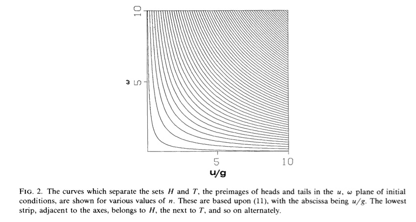
Fig. 1 From The Probability of Heads by Keller (1986).

What Keller shows is that while a coin flip is an entirely deterministic process, the outcome is uncertain due to an inability of any human (or machine!) to prescribe the initial conditions in such a way as to reliably get a heads or tails. Fig. 1 shows the outcome of a coin toss for an initial angular velocity, \(\omega\), and vertical velocity, \(u\). The black lines denote the edges of regions of this parameter space that give rise to heads or tails. It’s not surprising that these bands alternate between heads and tails, but what is surprising is that the bands alternate increasingly rapidly as \(\omega\) and \(u\) increase. The bands become increasingly close together so that even the tiniest change in the spin or velocity of the coin will change it from a heads to a tails. This is an example of the concept of chaos, which is when the outcome of a system is enormously sensitive to initial conditions. (This is also known as the Butterfly Effect.) Bringing up this analysis serves to underline that even the most simple systems may need to be considered probabilistically, even if for no reason other than that the mechanistic description is less useful.

Flipping Several Coins

Accepting then that a coin is a random process, it may not yet be clear how we can learn much from flipping one coin at a time. In fact, one coin is not terribly exciting, but if we flip, say, \(N\) coins, things become much more interesting. Most obviously, flipping \(N\) coins has many more possible outcomes, from \(N\) heads to \(N\) tails and everything in between. If we want to write down the probability of observing say, 8 heads out of 20 coin tosses, we can take the likelihood of getting 8 heads and 12 tails: \(p^8(1-p)^{12}\). (Why does this formula make sense?) However, there are many ways to get 8 H and 12 T, the first 8 flips can all be heads and the last 12 can all be tails, or the first 7 can be heads and the next 12 tails and the last a heads again, etc. To account for this we use the combinatorial factor \({20 \choose 8} = \frac{20!}{8!12!}\), where the “!” is the factorial operator (\(5!=5\cdot4\cdot3\cdot2\cdot1\), for example).

Writing the above more generally, we get

(3)\[P(k\text{heads in}N\text{flips of a coin}) = P(k|N, p) = \frac{N!}{k!(N-k)!}p^k(1-p)^{N-k},\]

which you may recognize as the binomial distribution. We have not yet discussed distributions, but they are the central concept to this entire text. Most broadly, a probability distribution or Probability Density Function (PDF) can be understood as a description of how specific outcomes of a random variable are distributed (how the density of probability is spread out). So in the case of a single coin with \(P(X=H)=p\), the PDF is written

\[\begin{split}P(X=x) = \begin{cases} p\qquad&x=H\\ 1-p\qquad&x=T \end{cases}\end{split}\]

to explicitly state the coin flip distribution. The binomial distribution then describes how the different number of heads in \(N\) coin flips are distributed.

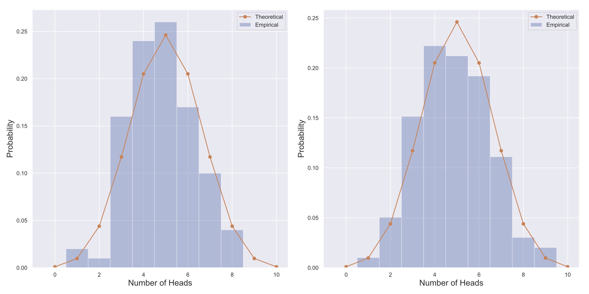
Fig. 2 Visualization of two empirical distributions generated from flipping 10 fair coins 100 times. The theoretical binomial distribution is plotted over each in orange.

Probability distributions, loosely speaking, come in two flavors: empirical and theoretical. Empirical PDFs (ePDFs) are of the kind that you’ll generate in the worksheets and problem sets; generated from a finite amount of data and proportional to a frequency distribution. Theoretical probability distributions instead (usually) have a closed mathematical formula, and can be thought to represent the limiting empirical distribution in the case where you have infinite data. An example of each can be found in Fig. 2 where two different instances of an empirical distribution are shown as the blue bars and a theoretical PDF is shown by the orange line in each panel. As an analogy, the difference between empirical and theoretical probability distributions is similar to the difference between the equation of a circle, \(x^2+y^2=1\), and any real world drawing of a circle. The real world drawing approximates the circle, and there are ways to improve this approximation, but the equation is always a Platonic ideal that cannot be achieved due to the finite nature of the physical universe. Similarly, repeated constructions of an empirical probability distribution will result in slightly different approximations to the ideal, as can be seen in Fig. 2.

While this may sound somewhat philosophical, it is crucial to understand that any real world measurement is an empirically acquired outcome of some random process, and therefore will change upon repeated observation. Hopefully you can see that while we would ideally like to make many observations, so as to put ourselves closer to the regime of the theoretical distribution, this is obviously not always the case. In fact, it is relatively common to find ourselves in the data-poor limit of an experiment, so it’s very important to be especially cognizant of the fact that we have empirical observations. As an example, if you toss a fair coin 10 times, it is very possible to get 8 heads (this should happen \(\sim5\%\) of the time according to Equation (3)!). If you were to then assess that the coin is biased, you would be wrong! The goal of of probability and statistics is to help you separate what is signal from what is noise by allowing you to assess the likelihoods of different outcomes.

Features of Distributions

One of the most fundamental insights in all of science is that while the outcome of a single experiment, say a single coin toss, is uncertain, there is a regularity to the outcome of many experiments. You will see this play out in the worksheets and assignments, but you should also recognize this from your own life; if you were to measure a table’s length with a ruler and get 1.8 meters, and then you measured it again, you would not get 12 meters. You may however get 1.81 or 1.79 meters depending on how you angled your ruler. If you made many measurements of the table’s length, you would probably get a very narrow distribution of table lengths centered at 1.8 meters, and you would be very justified in reporting that the table is 1.8 meters long.

This may seem somewhat trivial, but the point is this: we’ve elaborated that measurements are random events where the likelihood of any outcome has some (unknown) distribution, and we’ve noted that repeated observations allow us to get closer to a theoretical distribution, so when we are taking measurements of some quantity, we’re not trying to get a better list of numbers, we’re trying to discover the underlying distribution that governs how a quantity is observed. That is, we want to know about a quantity’s probability distribution in order to characterize it. Furthermore, we can assert that all quantities are actually distributions from which we draw observations.

While this may seem somewhat abstract - and it is - what it means to you as a quantitative thinker is that we should be very concerned with the shape of our observations’ probability distribution. It may not be clear why we can expect our observations to have any regularity, and we’ll get to that shortly, but for now, let’s discuss what sort of features of our distributions are interesting.

Moments of Distributions

Perhaps most obviously, we might be interested in the most frequent outcome of a random event (this is known as the mode of the distribution). For example, if you were given a coin with an unknown bias, you can imagine conducting many experiments of many coin flips and looking at what the most frequent result was to determine whether the coin is fair or not. That is, we can potentially (hopefully) infer the fairness of the coin by observing properties of its probability distribution.

However, as we’ll show in assignments and in later sections, looking at peaks of distributions is not the only useful feature. For example, consider Fig. 2, in which the distributions for the number of heads in 10 coin flips are shown after performing the experiment (10 coin flips) 100 times. According to the left panel, the mode is 5 heads (in 10 flips), and according to the right panel, the mode is 4 flips. If we had only this information, it would be very hard to know whether the same coin was used to generate the distributions (it was!).

In fact, there are some general mathematical ways to quantify different features of a distribution. In particular, we can talk about the mean or expectation of a distribution, which can be calculated either from a theoretical probability distribution

\[E[X] = \int_{x\in X}xP(X=x)dx,\]

or from an empirical distribution

(4)\[E[X] = \sum_{x\in X}xP(X=x),\]

where \(\Sigma\) is the summation operator, so we want to add up \(x\) times \(P(X=x)\) for all possible values of \(x\). So for example, if we consider \(X\) to be the roll of a fair die, then \(x\) can be either \(1, 2, 3, 4, 5, \) or \(6\) and the full sum can be written

\[\begin{align*} E[X] &= (1)\cdot P(X=1) + (2)\cdot P(X=2) + (3)\cdot P(X=3)\\ &\qquad\qquad + (4)\cdot P(X=4) + (5)\cdot P(X=5) + (6)\cdot P(X=6) \\ &= 1\cdot\frac{1}{6} + 2\cdot\frac{1}{6} + 3\cdot\frac{1}{6} + 4\cdot\frac{1}{6} + 5\cdot\frac{1}{6} + 6\cdot\frac{1}{6} = 3.5, \end{align*}\]

and we expect the value of the die to yield 3.5 on average. (Make sure this makes sense to you!) Note that we talk about expected values of random variables, \(X\), not particular outcomes (\(x=1\), for example); the outcome of a random variable is uncertain, but if the die came up 1, then that’s our value.

If we think of the mean as a measurement of a distribution’s center, how can we describe its width? One measure of “width” is the variance, which can be calculated

(5)\[Var[X] = E[(X-\mu)^2] = E[X^2] - E[X]^2,\]

where \(\mu = E[X]\) and \(E[X^2] = \sum_{x\in X}x^2P(X=x)\). Using this formula, we find that the variance of a single die roll is

\[Var[X] = 1\cdot\frac{1}{6} + 4\cdot\frac{1}{6} + 9\cdot\frac{1}{6} + 16\cdot\frac{1}{6} + 25\cdot\frac{1}{6} + 36\cdot\frac{1}{6} - (3.5)^2 = \frac{91}{6} - (3.5)^2 = 2.9167.\]

The standard deviation of a set of observations is another common measure of spread and is defined as the square root of the variance (\(\sigma = \sqrt{Var[X]}\)).

You can imagine that there are a whole set of measurements \(E[(X-\mu)^n]\), and indeed, these are called the moments of a distribution (\(E[(X-\mu)^n]\) is the \(n^{\text{th}}\) moment). In fact, as \(n\) increases, you learn about the shape of the distribution further and further from the mean. Specifically, the odd values of \(n\) give information about how asymmetric the distribution is and the even values about how symmetric the distribution is. A certain version of \(n=3\) is called the skewness and \(n=4\) is known as the kurtosis of the distribution.

Try It Yourself

To put this theory into practice, take a stab at Worksheet 1.1.

Once you have completed this worksheet, you should have enough practice to start to work on Assignment 1!

Cumulative Distribution Functions

One important note to make here is that when we have empirical distributions, we need to be careful about how we define \(P(X)\). Say for example, you were measuring the heights of everyone at Northwestern, but rather than keeping track of thousands of heights, you were just counting how many people’s heights fell into a set of bins, e.g. 120cm-130cm, 130cm-140cm, etc. (Would this be a distribution??) As you’ll explore in worksheets and assignments, your choices as to bin size and number will affect any calculations of moments that you make later on.

Try It Yourself

Change the bin sizes in your histograms and distributions in Worksheet 1.1. That is, instead of showing how many times you observed 5 heads, 6 heads, 7 heads, etc. Show how many times you observed 0, 1, or 2 heads, the number of times you observed 3, 4, and 5 heads, etc. How do any calculations based on the PDF change? Try and modify any curves generated using *theory} to use the same bins.

While this is not catastrophic, it’s also not desirable, so it is worth noting that we can also characterize the shape of a distribution using percentiles. A percentile is defined as the value of an observation such that a certain percent of all the observations are less than or equal to that value. More formally:

\[Q_X(p) = \min_{x\in X}\left\{x \left| \sum_{\chi \leq x}P(X=\chi) \geq p\right. \right\}\]

To calculate percentiles empirically, we will want to generate a cumulative distribution function, or CDF (we’ll sometimes denote an empirical CDF as eCDF to distinguish from theoretically derived CDFs):

\[F[x] = \int_{-\infty}^xP(X=x)dx.\]

In words, the CDF describes the likelihood of getting an outcome less than \(x\), and as such is also sometimes written \(P(X\leq x)\). We can do this empirically using the following Python code:

import collections

## Counts the number of times each value in data is seen 
counts = collections.Counter(data)  
                                
## Gets unique values of data and sorts
vals = np.msort(list(counts.keys()))    

## List comprehension to get ordered counts for each value
## cumsum then cumulatively sums these counts
CDF = np.cumsum(np.array([counts[ii] for ii in vals]))

## Normalize so that the PDF adds to 1.
CDF = CDF / CDF[-1]

Using this code, we can generate CDFs for the data shown in Figure Fig. 2, which are shown in Fig. 3. Then, using the CDFs, we can easily read off percentiles by finding the desired percentile on the \(y\)-axis and finding the corresponding \(x\)-coordinate on the CDF. For example, in Figure \ref{fig:TwoEmpCDFsBinom}, we can see that the 20th percentile of both distributions is approximately \(k=3\) heads.

Try It Yourself

Use the above code to make CDFs of the distributions in Worksheet 1.1.

Particularly interesting quantities are the median, which is the 50th percentile, and the Inter-Quartile Range (IQR), which is the distance between the 25th and 75th percentiles (the first and third quartiles). In both the examples in Fig. 3, the median and IQR are 5 and 2, respectively. The median and IQR are often more useful for characterizing a distribution than the mean and variance because they are robust to outliers in your observations.

Fig. 3 Empirical and theoretical CDFs for the number of heads in 100 experiments of 10 coin tosses. Note that in neither of the 100 experiments was 0 heads observed, so neither empirical CDF extends to \(x=0\). Similarly, in the left panel’s 100 experiments, no observations of 9 or 10 heads were made either. The median, 25th, and 75th percentiles are also shown, and the IQR is indicated.

It’s worth mentioning that while the binomial distribution is a useful and intuitive distribution to know, it is certainly not the only theoretical distribution worth knowing about. In particular, Normal or Gaussian distributions and Poisson distributions are often useful in quantitative analyses. However, their functional forms are not essential for the understanding of the main part of this chapter, so we will leave them to the end.

Try It Yourself

Use numpy.random.randn to generate 2 lists of 10 normally distributed random numbers. Add the value 100 to one of the lists. Compare the mean and median of the 2 lists. Which is the better descriptor of the “average” value of the list, the mean or median?

The Central Limit Theorem

In the previous sections, we’ve mentioned that theoretical distributions are the infinite-data limit of observational (sampling) distributions, but we have not provided any rigorous reason why our approximations get better as we make more observations. We will not do so here except to highlight the famous Central Limit Theorem (CLT), whose many proofs provide the basis for our assertion. We will not prove the CLT here, instead we find it most useful just to highlight its main result and assumptions.

Specifically, the CLT says that in an extraordinary number of cases, the ratio of the standard deviation (\(\sigma\)) to the mean (\(\mu\)) of a set of observations decreases as the number of observations, \(N\) is increased. Moreover, the ratio decreases in a specific fashion: as the square root of \(N\), as shown below.

(6)\[\frac{\sigma}{\mu}\sim \frac{1}{\sqrt{N}}\]

More intuitively, if we think of the mean as a measure of the “center” of our distribution, and the standard deviation as the error in estimating the true mean, then our ability to estimate the first moment of our distribution increases as the number of data points is increased.

Now you might see how this could be useful. If we’re concerned about separating signal (\(\mu\)) from noise (\(\sigma\)), then we can use the CLT to determine exactly how many observations we need to estimate the mean to a certain accuracy. However, the CLT requires a few assumptions about the data in order to make this statement:

• all measurements are independent of one another, and

• all observations must be generated from the same underlying process. In terms of a coin toss, as long as each coin being tossed has the same value for \(P(X=H)=p\), then tossing increasing numbers of coins improves our empirical estimation of \(p\). That is, the CLT tells you that if you continue flipping a coin enough times, you can be increasingly confident calculating \(p\). Hopefully this is reassuring and intuitive: adding more data should improve our inferences and estimates.

Try It Yourself

Consider the experiment from Worksheet 1.1 where you are flipping \(N\) coins repeatedly. If I want the standard deviation in the number of heads to be on average 10% of the mean, how many coins do I have to flip? Show this with code if you can (or if you’re having trouble with the theory)!

The flipside of this is that when we have very few measurements of a phenomenon, then our ability to estimate a given feature of the distribution, say the mean, will be error-prone. The CLT tells us that the error in these estimates will often scale with the inverse square root, as shown in Equation (6), but that is not much comfort if we only have 2 or 3 measurements. This is worth keeping in mind whenever you are working with data, even if it is “big”; there is a difference between having a few measurements of many different quantities and many measurements of just one quantity.

If this were all the CLT gave us, it would be a useful result, but the CLT also can be stated (in combination with the Law of Large Numbers) to say that if you have enough measurements (if \(N\) is big) of an independently and identically distributed (i.i.d.) random variable, then the distribution of the mean of those measurements can be characterized completely with only the mean and standard deviation (the first two moments) of the random variable. For those with some previous experience in these topics, the CLT says that the sum of i.i.d. random variables becomes a Gaussian distribution as the number of observations, \(N\), increases. Even more specifically, if the i.i.d. random variables have mean \(\mu\) and standard deviation \(\sigma\), then the distribution of the mean has mean \(\mu\) and standard deviation \(\sigma/\sqrt{N}\). This may seem like an odd thing to focus on but it’s actually very useful as we now know how any sum of i.i.d. variables is distributed. While in most of this course we will stay away from making assumptions as to the form of any distribution, it is quite remarkable that all sums of random variables are distributed similarly.

The upshot of the CLT is this: when the assumptions are met, it is a very useful result! However, in many situations we do not have many i.i.d. random variables, so it is not prudent to preoccupy oneself only with analyses that rely on the CLT to work. Instead, we hope to build up some methods that will apply even when the assumptions of the CLT are not strictly valid.

Try It Yourself

Try your hand at Worksheet 1.2. You should also now be able to attack most of Assignment 1!

The Atom of Bayesian Probability

Throughout this text, our goal is to remove obstructing details and formulas from your path towards becoming a quantitative worker. While some details are inevitably necessary in any field, what we have been emphasizing are the most important and most useful parts of theory for actually learning things from data. If you have previously taken a statistics course, it may come as a surprise to you then that we think it’s worthwhile to talk about Bayes’ Theorem. Our motivation here is partly philosophical, but also (as always) practical.

First, Bayes’ Theorem can be written explicitly:

(7)\[P(A | B) = \frac{P(B | A)\cdot P(A)}{P(B)}.\]

As noted earlier, the expression \(P(A | B)\) is read “the probability of random event \(A\) *given} random event \(B\)” and is called a **conditional probability}. This name is due to the fact that we are thinking about the likelihoods of outcomes of random event \(A\) conditioned on (depending on) the outcome of random event \(B\). In this way, Bayes’ Theorem is simply a formula relating the conditional probabilities of two random events.

Try It Yourself

Using Equation (2) in two symmetric ways, see if you can derive Bayes’ Theorem yourself.

To make it clear why Bayes’ Theorem might be useful, let’s consider random event \(B\) to be the act of observing data and random event \(A\) to be some interesting feature of the data distribution, let’s say the mean. Then as a data researcher, we might be concerned with knowing that interesting feature, and if we’re being careful, we might be very concerned with how well we can know that feature given that we collected certain data. That is, we are almost always concerned with knowing \(P(\text{FEATURE}|\text{DATA})\), the likelihood that our feature has a specific value given our specific data. This quantity is known as the posterior distribution for the feature \(A\).

(8)\[P(FEATURE|DATA) = \frac{P(DATA|FEATURE) P(FEATURE)}{P(DATA)}\]

The reason then that Bayes’ Theorem is so appealing is that it gives us an explicit structure in which to calculate this conditional likelihood. Specifically, if we can construct the parts of the right-hand side of Equation (7), we can plug them into Bayes’ Theorem and we have our answer. You may be concerned however as to how we might know the parts of the right-hand side better than the left, and this is a main criticism of Bayesian statistics, however Bayesian practitioners prefer to keep their assumptions front and center (as a main part of any calculation), than not. But before we get into the philosophical side, what even is on the right-hand side of this equation?

Keeping the analogy that \(A = \)FEATURE and \(B = \)DATA, then \(P(DATA|FEATURE)\) is the opposite conditional statement to the one we’re interested in, and is called the likelihood function. That is, it is the conditional likelihood of observing our data given some feature of the sampling distribution. In many cases (we’ll get into this), we have a model for how our data are generated, and this model may depend on some parameters, which may be features of a distribution. In any case, when we have such a model, Bayes’ Theorem accounts for it with this term.

The term \(P(A)\) is known as the prior and it represents our priorknowledge about how we think that the feature \(A\) is distributed before we collect any data. You may be inclined to assert that we don’t have any information about \(A\), otherwise we wouldn’t be doing experiments to measure it, but this isn’t really true - we often do have some guesses as to the shape or size of \(A\). For example, if I hand you a coin and tell you it’s from the U.S. Mint, it would not be entirely reasonable of you to state that you have absolutely no notion as to how often the coin will land on heads. Based on personal experience alone, it would be more prudent to start from the assumption that the coin is probably fair and wait for new evidence to convince you otherwise. It’s worth mentioning that even if you want to insist that you don’t know anything, you can often plug in what is called a non-informative prior, for example, a uniform distribution for \(p\) from 0 to 1 in the case of the coin toss. Also, regardless of your choice of prior, given enough evidence Bayes’ Theorem will always converge to the same posterior distribution, so this seemingly arbitrary choice doesn’t often end up having that large of an impact. (We’ll explore this more concretely in a worksheet later.)

Let’s now work a specific example to see how this works.

Example: Bayesian Coin Tossing

While we’ll talk about parameter estimation more in the next section, let’s consider the scenario where you have been given a coin and you want to assess whether it is fair. We’ll use Bayes’ Theorem in a slightly looser formulation:

\[\begin{align*} P(p | k\text{ Heads in } N\text{ tosses}) &\propto P(k\text{ Heads in } N\text{ tosses}| p) \cdot P(p)\\ P(p| k, N) &\propto P_{Binom}(k|N, p) \cdot P(p), \end{align*}\]

where we omit the denominator, \(P(k\text{ Heads in } N\text{ tosses})\), because we know that the left-hand side is a probability distribution and thus must sum to 1. Let’s then say that \(P(p)\), our prior for the distribution of the heads probability, \(p\), is a uniform distribution from 0 to 1 (often denoted \(\mathcal{U}(0, 1)\)). That is, we’re asserting that we really don’t know anything about coins.

We know from our earlier derivation of the binomial distribution, that if we know \(p\), then we can write the likelihood of observing any number of heads \(k\) in \(N\) tosses is binomially distributed, so we write

\[P(k\text{ Heads in } N\text{ tosses}| p) = P(k|N, p) = {N\choose k}p^k(1-p)^{N-k},\]

which is the first factor on the right-hand side of Bayes’ Theorem.

Then, before we start flipping the coin, we can visualize our prior for the heads probability in Fig. 4. As a counter-point, we also consider a prior in which we strongly believe that the coin will be fair, with much less likelihood that it is biased. This is shown in Fig. 5. In this thought experiment, the coin actually is biased to have a heads probability of \(p=0.28,\) which is shown in the figures, but of course, we wouldn’t know this when we’re given the coin.

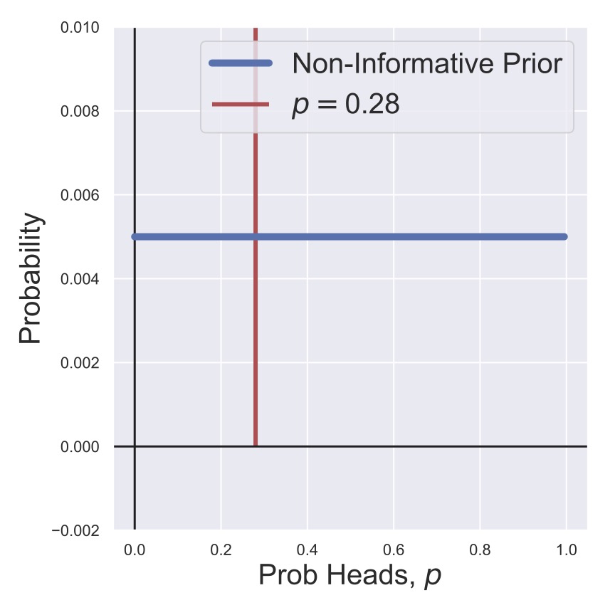
Fig. 4 A non-informative prior (uniform distribution).

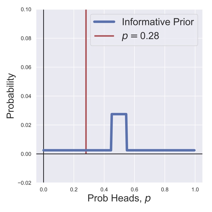
Fig. 5 An informative prior (non-uniform distribution).

In Fig. 6 and Fig. 7, we see the result of multiplying \(P(0 H | N=1, p)\) and our two priors \(P(p)\). That is, we flipped the coin and got a tails, so we shifted our estimates of the likelihood of heads away from \(p=1\) and towards \(p=0\), although in the case of our informed prior we’re still holding out considerably for a fair coin.

That is, we’re showing the function given by

\[f(p) = P_{Binom}(k{=}0|N{=}1, p) \times P(p),\]

for two different choices of \(P(p)\) (as shown in Fig. 4 and Fig. 5).

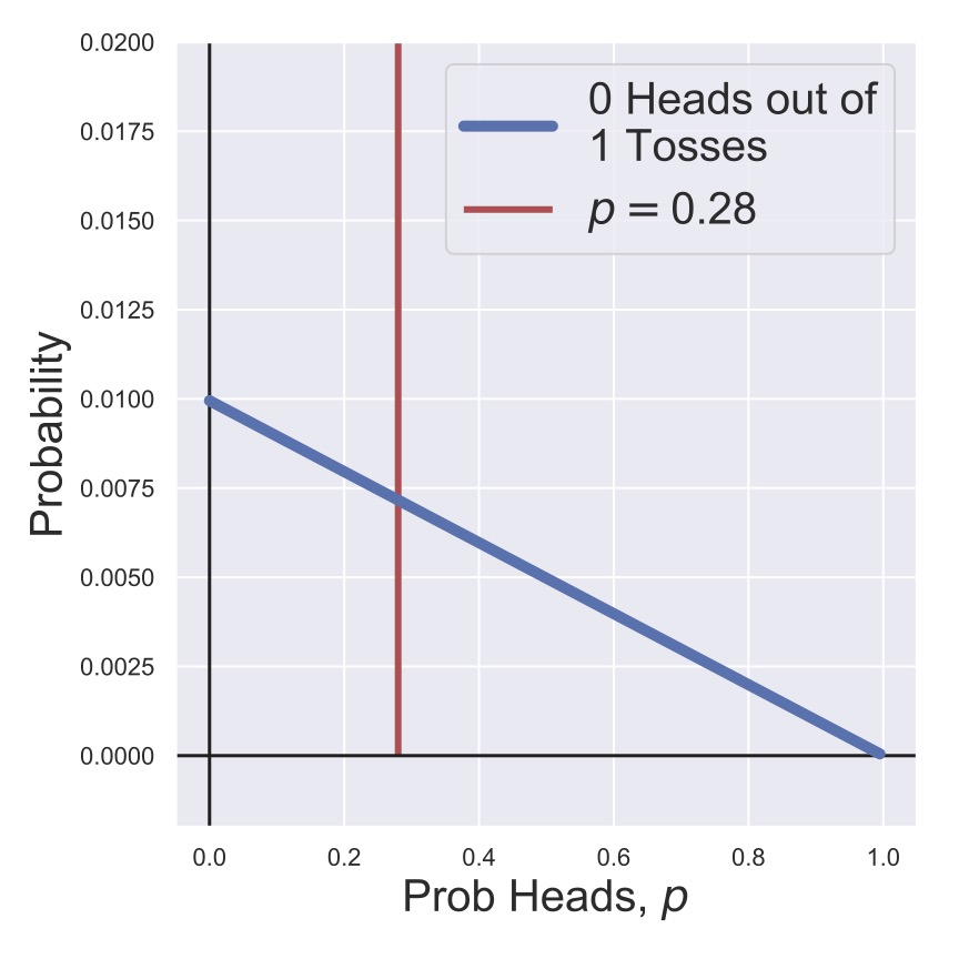
Fig. 6 A posterior distribution for the heads probability of a coin after one toss with a non-informative prior.

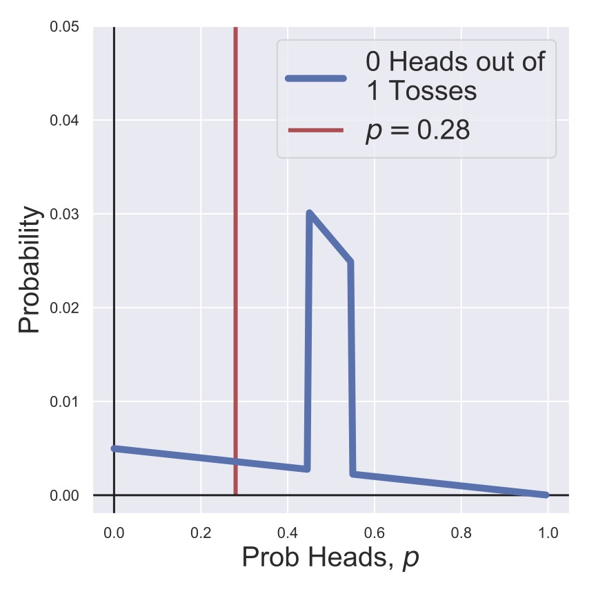
Fig. 7 A posterior distribution for the heads probability of a coin after one toss with an informative prior.

In Fig. 8 and Fig. 9, we’ve flipped two coins, one of which is a heads, so the posteriors have recentered themselves on \(p=0.5\). Then in Fig. 10 and Fig. 11, we’ve skipped ahead to flipping 10 coins, of which 9 were tails! Now we can see that both posteriors are starting to look similar, and the effect of our prior choice is becoming much less signficant.

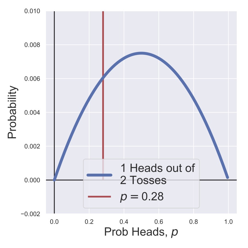
Fig. 8 A posterior distribution for the heads probability of a coin after two tosses with a non-informative prior.

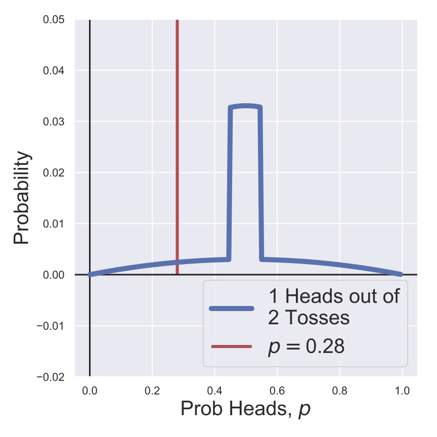
Fig. 9 A posterior distribution for the heads probability of a coin after two tosses with an informative prior.

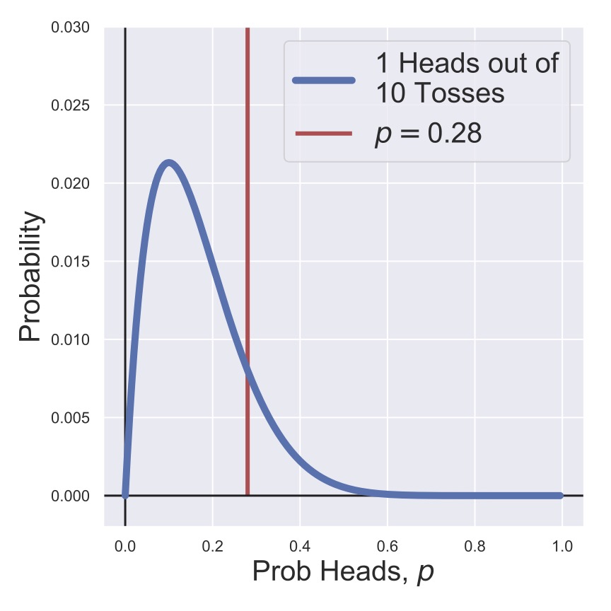
Fig. 10 A posterior distribution for the heads probability of a coin after ten tosses with a non-informative prior.

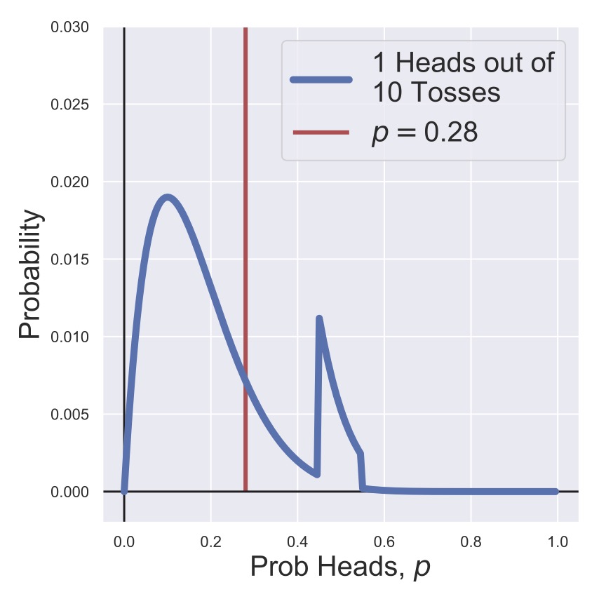
Fig. 11 A posterior distribution for the heads probability of a coin after ten tosses with an informative prior.

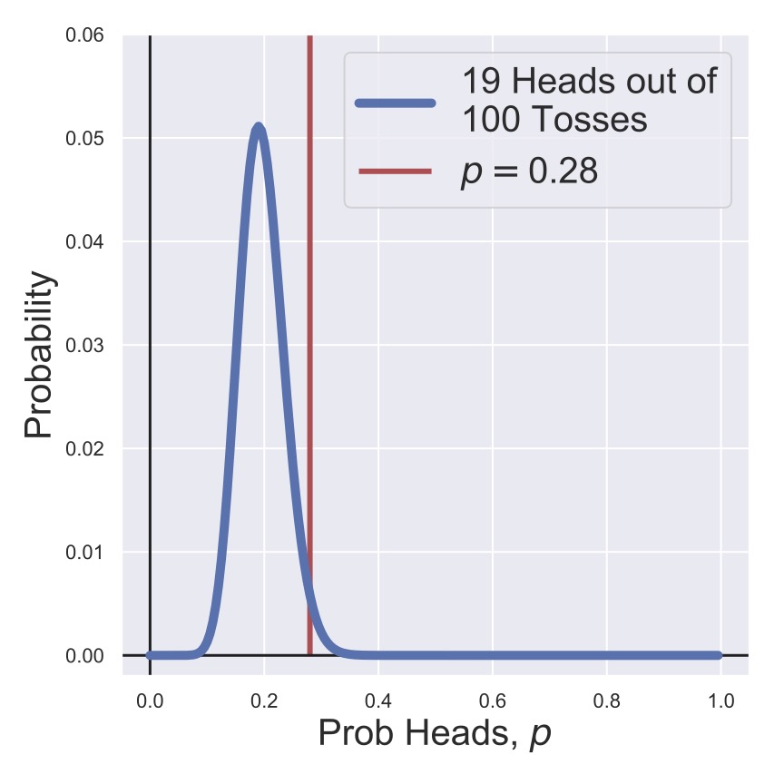
Fig. 12 A posterior distribution for the heads probability of a coin after one hundred tosses with a non-informative prior.

Fig. 13 A posterior distribution for the heads probability of a coin after one hundred tosses with an informative prior.

Finally, in Fig. 12 and Fig. 13, we have flipped the coin 100 times, so that any prior expectation for the heads probability is completely wiped out. Both posteriors are (very reasonably) centered on \(p=.19\) since we’ve observed 19/100 coins to be heads, but the true value of \(p=0.28\) still has a non-zero probability associated with it.

More explicitly, we’re showing the functions

\[f(p) = P_{Binom}(k{=}1|N{=}2, p) \times P(p),\]

\[f(p) = P_{Binom}(k{=}1|N{=}10, p) \times P(p),\]

and

\[f(p) = P_{Binom}(k{=}19|N{=}100, p) \times P(p).\]

Notice that each of these is a function of our parameter of interest, \(p\), only.

Try It Yourself

You now have the theoretical basis to make an attempt at Worksheet 1.3. Completing the worksheet will likely be necessary before attempting problem (3.f) on the assignment, so make sure you try the whole worksheet!

Why Bayes?

At the beginning of the section we described Bayes’ Theorem and how it might be conceptually useful, but the example in above also demonstrates a practical aspect of why Bayes’ Theorem is good to know: it gives us distributions for any features or parameters. We’ve spent most of this chapter discussing why individual observations should be considered probabilistically, meaning that they are samples from an underlying distribution, so a methodology that naturally is centered on this distributional way of thinking should be appealing.

We won’t probe all the nuances and uses of Bayes’ Theorem in this chapter, but we will make a point of showing how this relatively simple formula can be extended to most of the applications in this course. For now, we hope that you can start to see how Bayesianism dovetails nicely with a distributional mindset with regards to data; later we’ll show that Bayes’ Theorem is applicable very generally, even in cases where classical statistics breaks down.

Bacterial Chemotaxis

The first biological dataset you will be exploring is related to bacterial chemotaxis. There are beautiful texts (1, 2, 3, and 4, talks (1, 2, and 3), and papers on this topic. As is the theme of this course, we aren’t going to go into the details of topics related to biology, physics, or algorithms too deeply. We want to help you explore and extract information from data. We introduce chemotaxis here because it is a particularly clean biological system that produces data that can be analyzed using some of the tools we have already taught you. So, as a reference for the assignments, here is a very quick summary of the overall phenomenon.

Bacteria need to navigate the chemical landscape they inhabit - they need to move towards stuff they like, and away from stuff they don’t. This is called chemotaxis: chemically driven motion. In particular, if you place a source of sugar in a solution with bacteria, say a sugar cube, and the bacteria will move towards the sugar. While seemingly simple, over 50 years of genetics, molecular biology, and biophysics has gone into the study of this one phenomenon. Why? Not because its the most crucial biological phenomenon but because it’s a system where incredibly precise measurements and experiments can be performed. Fortunately, what we have learned have been incredibly general principals. Indeed, I could (and have) given an entire course in biophysics that solely focused on bacterial chemotaxis.

So, how do bacteria move in response to chemicals? As shown in Figure Fig. 14, they have oars, called flagella, that propel them through their surroundings. If you watch a single bacterium move you will see that they use their oars in a funny manner resulting in a path that looks like a series of straight lines interjected by abrupt turns, as shown in Figure Fig. 14. This particular method of movement is known as making runs and tumbles. The way in which the bacteria moves towards a sugar crystal is that on the occasions when the runs happen to point up the sugar gradient they tend to be longer. When the bacteria is pointed down the sugar gradient, the runs are shorter. This simple mechanism ensures that given random orientations after a tumble, the bacteria will have a net movement, averaged over the many runs and tumbles, towards the source of sugar.

So, what produces the runs and tumbles? Indeed the microscopic mechanism for this is rather straightforward. The bacteria has many oars, but instead of them being like the oars for a rowboat, they look like corkscrews. This may seem like a strange choice of oars but there is a very deep reason for this design (if you find this interesting make sure to delve into the books cited above, as well as this beautiful paper). Crucially then, a single bacteria has many of these corkscrew-oars. When the corkscrews spin in one direction (counter clockwise to the direction of motion) then bacteria moves in straight line, making a run. If they rotate clockwise the bacteria tumbles in place. This is shown in Fig. 15.

At this point then, the question is how a bacteria “knows” that it is moving up the gradient, and thus lengthen its straight line motion? Again, the answer to this involved around 2-3 decades worth of research, but one of the central experiments done to figure this out is what you will analyze as your first data set!

What researchers had difficulty with was in prescribing precise concentration profiles of chemicals and recording how bacteria modulated the frequency with which they did runs vs tumbles. So, to make the observations easier, some researchers chopped off the ends of the long flagella, and rooted the bacateria at the base of a flagellum down onto a slide. Now the bacteria couldn’t move translationally, but when the flagella rotated counter-clockwise (CCW) the bacteria would spin clockwise (CW), and vice versa. Now that the bacteria was spatially fixed, they could then pipette in very precise spatial profiles of chemicals and watch how the bacteria, now stuck in place, would respond. Watching a video of this is somewhat entertaining, but I hope you can appreciate how very simple experimental design choices can be the key to opening up decades worth of insights.

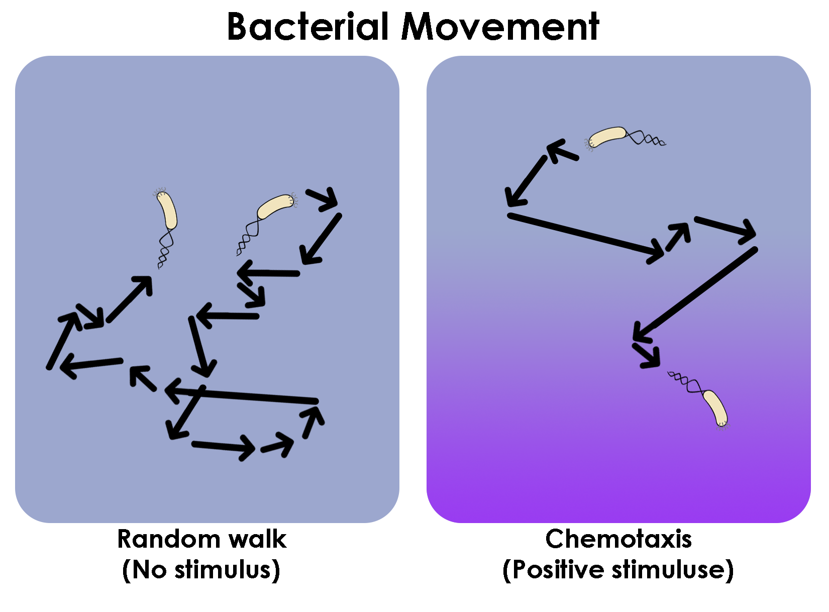
Fig. 14 The run-and-tumble trajectories of bacteria in two conditions: the absence of any stimulus (left) and in the presence of a positive stimulus gradient (right). Although it’s a cartoon, the idea is that there will be more runs that are longer in the direction of the gradient, compared to the movement when there is no stimulus.

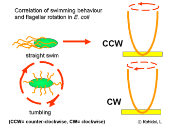
Fig. 15 An illustration of the physical arrangement of the flagella when they are rotated clockwise and counter-clockwise.

The data that you will be working with is the angular velocity of a bacteria that has been stuck to a slide. Your task in assignment 1 will be in part to verify that you see the bacteria attempting to run and tumble, and to show this phenomenon in a meaningful way. This data set has been taken from and some of the questions in the assignment have been inspired by William Bialek’s book on Biophysics, which I would thoroughly recommend for anyone interested in a more physical viewpoint of biology. Additionally, there is an entire set of notes we have written on chemotaxis that gives a lot more biological and physical background on the topic. Check it out if you are interested!

Review

So what was the point of this module? And why should you be reading this? How is this going to help you analyze your data?

A lot of the material here might be something you’ve seen before. However, getting some definitions and notations down is important. So I hope you have a more precise sense for what \(P(X=x)\) is saying. And, for example, how the conditional, marginal, and joint distributions are related to each other. Repeat these concepts in your mind over and over again, with simple examples (tossing two coins, drawing two cards with replacement from a pack, etc.) to really build intuition. I cannot emphasize enough that having these concepts deeply ingrained in your mind will serve you well.

Another really important idea was that even for something as simple as a coin flip you expect a variance in outcomes – a distribution. This makes estimating important features (which we introduced you to, such as the expectation or variance) from empirical data distributions challenging. At a more philosophical level, every statistic (quantity of interest), can only be determined to some finite precision from real data. You saw this in the simple example of coin flipping.

Please reflect on the depth of the central limit theorem within the context of coin flipping. I assure you that this fundamental result is playing a very important role in your data. Intuitively the CLT tells us why getting more data makes the accuracy of any statistic of your distribution better. Additionally, the CLT says that when you have lots of data then often the distribution becomes increasingly “well-behaved” – which means, it becomes increasingly Gaussian. Why do we say that Gaussian distributions are “well-behaved”? Because you can entirely describe a Gaussian distribution using only two numbers – its mean and its variance. And so you need only report two numbers to tell us everything we need to know about the distribution. Generically, the data you generate or want to analyze is actually not Gaussian, or you don’t have enough data, which makes characterizing it far more challenging, but we will teach you how to deal with this.

Finally, we briefly introduced a Bayesian point of view to give you some experience with the concepts of the prior, likelihood, and posterior distributions. These 3 can be combined via Bayes’ Theorem, which then allows one to exactly state your prior beliefs (the ones you held before you had any data), and update them in the face of new data. What is also beautiful about the Bayesian approach is that any parameter (the probability of heads, even) is now explicitly modeled in a distributional sense. As we’ll see in the next module, you won’t just get a single number for your estimate but always the whole probability distribution. Of course the price you have to pay is that you almost always need a theoretical formula for the likelihood function. (For coin flips we have the binomial distribution.) You’ll continue to encounter the Bayesian perspective as you continue in the course.

Learning Goals

To keep your expectations and goals in the right place, these are the skills and concepts we hope you have gained in the course of reading these notes, completing all the worksheets, and completing the assignment. After this module, you should be able to:

• Theory

  • Describe the concept of probability and random variables.

  • Interpret the notation \(P(X=x)\).

  • Define and interpret the joint, conditional and marginal distributions of two random variables.

  • Discuss theoretical and empirical probability distributions and the differences between them.

  • Explain why \(\int_{x\in X}P(X=x)dx = 1\)

  • Determine when two random variables are independent.

  • Discuss the Central Limit Theorem and its assumptions. Describe the \(\sqrt{N}\) rule.

  • Discuss Bayes’ Theorem and identify the components of Equation (7)

  • Discuss and interpret the Binomial Formula.

  • Discuss and interpret the definition of probability density functions and cumulative density functions.

• Calculations

  • Given some data (or a theoretical distribution), calculate: \(P(X=x)\), \(P(X\leq x)\), \(\sum_{x\in X}P(X=x)\).

  • Given data or a distribution, calculate \(E[X]\), \(Var[X]\), and other moments.

  • Given data or a distribution, calculate the median, IQR, or other percentiles.

  • Given data or a distribution, calculate the mode.

• Visualize

  • Plot empirical or theoretical PDFs and CDFs.

  • Use vertical or horizontal lines to show means, medians, and percentiles on PDFs and CDFs.

  • Show how different quantities change as a function of (simulated) parameters.

• Simulations and Coding

  • Simulate coin tosses with arbitrary \(N\) and \(p\).

  • Implement Bayes’ Theorem to calculate a posterior distribution.

  • Extract time intervals from a time series (Assignment 1).

  • Generate PDFs and CDFs from data.

In the worksheets and assignments you will implement and grapple with all of these ideas. Enjoy!

Other Details

More Probability Rules

Consider two random variables \(A\) and \(B\). Let \(a\) and \(b\) be specific outcomes of \(A\) and \(B\), respectively. The following are some mathematical rules that you can use to manipulate probabilities. These are absolutely not necessary to have memorized or accessible to be successful in this course, but thinking about them might help you gain some intuition about probabilities.

The Addition Rule

If we want to know the likelihood of either of two outcomes occurring, we can use the addition rule.

\[ P(A{=}a \text{ OR } B{=}b) = P(A{=}a) + P(B{=}b) - P(A{=}a \text{ AND } B{=}b)\]

The Multiplication Rule

We have already seen this in the notes, but this rule is sometimes called the multiplication rule:

\[\begin{split} P(A{=}a\text{ AND } B{=}b) &= P(A{=}a)\times P(B{=}b | A{=}a)\\ &= P(B{=}b)\times P(A{=}a| B{=}b).\end{split}\]

Notice the symmetry in the way this relation can be written.

The Complement Rule

This should be an obvious consequence of the fact that \(\sum_{x\in X}P(X{=}x) = 1\) (the likelihood of something happening is 100%), but this is formally called the complement rule.

\[ P(A{\neq}a) = 1 - P(A{=}a)\]

Law of Total Probability

We can always break probabilities of one random variable into conditional statements that depend on other random variables. This is explicitly done with the Law of Total Probability.

\[ P(A{=}a) = P(A{=}a|B{=}b)\cdot P(B{=}b) + P(A{=}a|B{\neq}b)\cdot P(B{\neq}b)\]

That is, the probability that \(A=a\) can be found conditionally by considering how likely it is when \(B=b\) and adding the likelihood that arises when \(B\neq b\).

Marginal Distributions

This previous rule suggests that we can extract probabilities of one random variable from a joint distribution. Indeed, if we want to know the probability distribution of \(A\) without consideration of \(B\), we can add up the way that \(A\) is distributed over all the different outcomes of \(B\). This is called marginalization and will come up later in the course. More concretely, if we have a joint distribution \(P(A, B)\), then we say that \(P(A)\) and \(P(B)\) are marginal distributions of \(A\) and \(B\). We can find these quantities from the joint using a summation (or integral):

(9)\[\begin{align} P(A) &= \sum_{b\in B}P(A, B)\\ P(B) &= \sum_{a\in A}P(A, B) \end{align}\]

More Theoretical Distributions

For the sake of clarity and brevity we ignored introducing the specific functional forms of some relevant and interesting distributions. We list them here with some relevant notes. Again, it is not necessary to memorize any of these formulas, and we will remind you of any relevant details as we go forward.

As a note about notation, probability distributions generally have parameters that determine their shape and moments. When we have a distribution of some quantity, \(x\), and it has parameters \(\theta_1, \theta_2, \ldots\), we will generally notate this distribution as

\[P(x;\theta_1, \theta_2,\ldots)\qquad \ProbOr\qquad P(x|\theta_1, \theta_2,\ldots).\]

It may seem odd that we’re re-using the notation for conditional probabilities, but you can convince yourself that the notation we’re trying to express actually is a conditional probability – we’re conditioning on the different parameters.

The Binomial Distribution

We have already discussed this extensively in the text, but the binomial distribution describes the distribution of the number of successes, \(k\), that occur in \(N\) trials, where the likelihood of a single success is \(p\). If a “success” is a coin coming up heads, then this distribution describes the number of heads in \(N\) flips of a coin.

The formula for the PDF is given by Equation (3), which we repeat here:

\[ P_{Binom}(k;N, p) = {N\choose k}p^k(1-p)^{N-k}.\]

In the scipy.stats package, you can access the binomial distribution with the scipy.stats.binom object.

The Gaussian Distribution

Perhaps the most important distribution ever, the Gaussian or Normal distribution describes a wide variety of phenomena. We’ll discuss it increasingly as the course progresses, but for now we’ll just give some basic facts.

Normal distributions are parameterized by their mean, \(\mu\), and variance, \(\sigma^2\), which should be interesting on its own. The PDF is given by

\[ P_{Gauss}(x;\mu, \sigma^2) = \mathcal{N}\left(x;\mu,\sigma^2\right) = \frac{1}{\sqrt{2\pi \sigma^2}}e^{-\frac{(x-\mu)^2}{2\sigma^2}}.\]

When \(\mu=0\) and \(\sigma^2=1\), the distribution is referred to as the standard normal distribution. You can convert any normal distribution to a standard normal by making the substitution \(y = (x - \mu)/\sigma\) (subtracting the mean and dividing by the standard deviation). This is known as standardization.

In the scipy.stats package, you can access the binomial distribution with the scipy.stats.norm object.

The Poisson Distribution

The Poisson distribution is another useful distribution to know about as it arises frequently in natural processes. It describes the distribution of events that occur in a given time interval, if the average number of events in an interval is \(\lambda\) (also known as the arrival rate), and each event occurs independently of the last. The Poisson distribution can be considered to be a limiting case of the binomial distribution when the probability of success is very small.

The PDF of the Poisson distribution is

\[ P_{Poisson}(k;\lambda) = \frac{\lambda^ke^{-\lambda}}{k!}\]

In the scipy.stats package, you can access the binomial distribution with the scipy.stats.poisson object.

The Exponential Distribution

Finally, the exponential distribution describes random variables whose PDFs are exponential functions. You will explore the exponential distribution extensively in the assignments, so for now we will only say that the exponential distribution can be used to describe the time interval between Poisson-distributed events.

The PDF of the exponential distribution is

\[\begin{split} P_{Expon}(x;\lambda) = \begin{cases} \lambda e^{-\lambda x} &\qquad x\geq 0\\ 0 & \qquad x < 0 \end{cases}\end{split}\]

In the scipy.stats package, you can access the binomial distribution with the scipy.stats.expon object.